+ 기출 형변환
import pandas as pd
df = pd.DataFrame({'rating': ['1', '2', '4', '*7', '8', '*7', '3', '5', '2', '*4']})
df.info()
*이 섞여있어서 object 타입으로 나옴
#해결방법
df['rating'] = df['rating'].replace('\*', '', regex=True).astype('int')
df.info()
-> int64로 변환 성공
고객 구매 데이터를 사용,
고객이 주문한 물품이 제 시간에 도착하는지 도착여부(Reached.on.Time_Y.N) 예측
1. 데이터 읽어오기
1) 사용 lib 및 환경 설정
#lib import
import pandas as pd

#max_rows max_columns 지정
pd.set_option('display.max_rows',500)
pd.set_option('display.max_columns',20)

#출력 format 지정 (.4f)
pd.set_option('display.float_format', '{:.4f}'.format)
2) x_train, x_test 데이터로 생성
from sklearn.model_selection import train_test_split
dftot = pd.read_csv('./bigdata/1st_Train.csv')
x_train, x_test = train_test_split(dftot, test_size=0.4,
		stratify=dftot['Reached.on.Time_Y.N'],
		random_state=0)
y_train = x_train[['ID', 'Reached.on.Time_Y.N']]
x_train = x_train.drop(columns=''Reached.on.Time_Y.N')
y_test = x_test[['ID', 'Reached.on.Time_Y.N']] #시험에선 제공 X
x_test = x_test.drop(columns='Reached.on.Time_Y.N')

x_train.to_csv('x_train.csv', index=False)
y_train.to_csv('y_train.csv', index=False)
x_test.to_csv('x_test.csv', index=False)
y_test.to_csv('y_test.csv', index=False) #시험에선 제공 X

x_train.shape, y_train.shape, x_test.shape
#((6599, 11), (6599, 2), (4400, 11))
3) 데이터 읽어오기
X = pd.read_csv('x_train.csv')
Y = pd.read_csv('y_train.csv')
X_submission = pd.read_csv('x_test.csv')
print(X.shape, Y.shape, X_submission.shape)
#(6599, 11) (6599, 2) (4400, 11)
4) X, X_submission concat (필수는 아닌데 같은 전처리를 편하게 하기 위해)
dfX = pd.concat([X, X_submission], axis=0, ignore_index=True)
print(dfX.shape) #(10999, 11)

#axis=0 생략 가능
5) 정보 확인
dfX.info()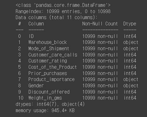
> 결측치 0 object type 4개
2. 전처리
1) 데이터 점검
#결측치 점검
print(dfX.isna().sum())
#결측치 : 0


#상관관계 확인
print(dfX.corr())
#1이나 -1과 가까운 값이 없어서 모든 Feature사용 가능


#Y값의 분포 확인
temp = Y['Reached.on.Time_Y.N'].value_counts(normalize=True).sort_index()
print(temp)
# 0 : 40.32% (제 때 도착X),   1 : 59.68% (제 때 도착O)
#normalize=True / 비율로 확인 가능
#sort_index 생략 가능
2) X, Y 합치기
X.columns, Y.columns
# ID 컬럼 항목이 겹치는 것을 알 수 있음
# 그래서 concat 말고 merge 사용

#dfX = X + X_submission > shape -> 10999, 11
#X.shape -> 6599,11

dfXY = pd.merge(dfX.iloc[:6599, :], Y)
#dfXY = pd.merge(X, Y)
print(dfXY.shape) # (6599,12)
3) 범주별 'Reached.on.Time_Y.N'의 개수, 비율을 표시하는 DataFrame 작성 함수
def make_table(df, feature):
	result = pd.DataFrame()
    temp = df.groupby([feature, 'Reached.on.Time_Y.N'])[feature].count()
    result['Count'] = temp

    sList = []
    for k in sorted(df[feature].unique()):
    	temp = df.loc[df[feature]==k, 'Reached.on.Time_Y.N'].value_counts(normalize=True)
        temp = temp.sort_index()
        sList.append(temp)
    result = result.reset_index()
    result['Rate'] = pd.concat(sList, ignore_index=True)
    return result
4) 대입해서 개수, 비율 알아보기
#'Warehouse_block', 'Reached.on.Time_Y.N'별 'Warehouse_block'의 개수, 비율
temp = make_table(dfXY, 'Warehouse_block')
print(temp)
# A B C D F

#'Mode_of_Shipment', 'Reached.on.Time_Y.N'별 'Mode_of_Shipment'의 개수, 비율
temp = make_table(dfXY, 'Mode_of_Shipment')
print(temp)
# Flight Road Ship

#'Product_importance', 'Reached.on.Time_Y.N'별 'Product_importance'의 개수, 비율
temp = make_table(dfXY, 'Product_importance')
print(temp)
# high low medium

#'Gender', 'Reached.on.Time_Y.N'별 'Gender'의 개수, 비율
temp = make_table(dfXY, 'Gender')
print(temp)
# F M

#dfX의 각 컬럼의 값 종류 개수 (1인 것 제거하기 위해)
dfX.nunique()
5) Object 타입에 대한 Label Encoding => de_LE
#Label Encoding
df_LE = dfX.copy()
df_LE['Gender'] = dfX['Gender'].replace(['F', 'M'], [0, 1])
df_LE['Warehouse_block'] = dfX['Warehouse_block'].replace(['A', 'B', 'C', 'D', 'F'], [0, 1, 2, 3, 4])
df_LE['Mode_of_Shipment'] = dfX['Mode_of_Shipment'].replace(['Ship', 'Road', 'Flight'], [0, 1, 2])
df_LE['Product_importance'] = dfX['Product_importance'].replace(['low', 'medium', 'high'], [0, 1, 2])
df_LE.info()
6) Object 타입에 대한 One Hot Encoding => de_OH
features = ['Warehouse_block', 'Mode_of_Shipment', 'Product_importance'] #ObjectTypeFeatures
df_OH = dfX.copy()

#Gender은 값이 두개라 Label Encoding 사용
df_OH['Gender'] = dfX['Gender'].replace(['F', 'M'], [0, 1])
#int type만
df_OH = df_OH.drop(columns=features)

tempList = [df_OH]
for f in features:
	s = pd.get_dummies(dfX[f])
    # s = dfX[f].str.get_dummies() 와 동일함
    tempList.append(s)
df_OH = pd.concat(tempList, axis=1)
print(df_OH.shape) #(10999, 19)
print(df_OH.columns)
#Index(['ID', 'Customer_care_calls', 'Customer_rating', 'Cost_of_the_Product',
#       'Prior_purchases', 'Gender', 'Discount_offered', 'Weight_in_gms', 'A',
#       'B', 'C', 'D', 'F', 'Flight', 'Road', 'Ship', 'high', 'low', 'medium'],
#      dtype='object') // 값들이 컬럼이 된걸 볼 수 있음
# 하나씩 하지 않고 한꺼번에 OneHotEncoding!
df_OH = dfX.copy()
df_OH['Gender'] = dfX['Gender'].replace(['F', 'M'], [0, 1])
df_OH = pd.get_dummies(df_OH)
print(df_OH.shape)
print(df_OH.columns)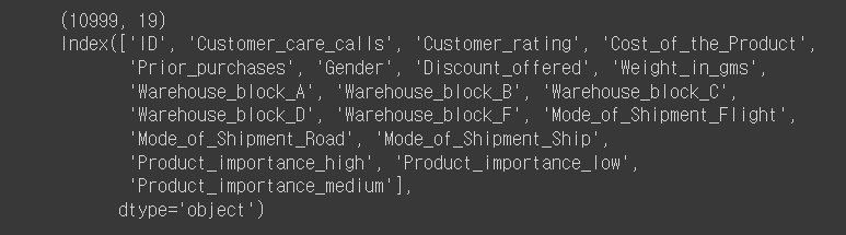
df_OH에서 영향력 없어보이는 컬럼은 제거하고 있는 컬럼만 골라서 사용
features = ['ID', 'Customer_care_calls', 'Customer_rating', 'Cost_of_the_Product',
       'Prior_purchases', 'Discount_offered', 'Weight_in_gms', 'A',
       'B', 'Flight', 'Road', 'high']
df_MINI = df_OH[features]
3. 데이터 분리, 모델 생성 및 학습
1) 사용할 도구 import
from sklearn.preprocessing import MinMaxScaler
from sklearn.model_selection import train_test_split
from sklearn.linear_model import LogisticRegression
from sklearn.neighbors import KNeighborsClassifier
from sklearn.tree import DecisionTreeClassifier
from sklearn.ensemble import RandomForestClassifier
from xgboost import XGBClassifier
from sklearn.metrics import roc_auc_score
2) score(train, test, roc_auc) 반환 함수
def get_scores(model, xtrain, xtest, ytrain, ytest):
    A = model.score(xtrain, ytrain)
    B = model.score(xtest, ytest)
    ypred = model.predict_proba(xtest)[:, 1] #1에 대한 값
    C = roc_auc_score(ytest, ypred)
    return '{:.4f} {:.4f} {:.4f}'.format(A, B, C)
3) 다양한 모델을 만들고 성능을 출력하는 함수
def make_models(xtrain, xtest, ytrain, ytest):
	model1 = LogisticRegression().fit(xtrain, ytrain)
    print('model1', get_scores(model1, xtrain, xtest, ytrain, ytest))

    for k in range(1, 10):
    	model2 = KNeighborsClassifier(k).fit(xtrain, ytrain)
        print('model2', get_scores(model2, xtrain, xtest, ytrain, ytest))

    #overfitting 트리
    model3 = DecisionTreeClassifier(random_state=0).fit(xtrain, ytrain)
    print('model3', get_scores(model3, xtrain, xtest, ytrain, ytest))

    #overfitting해결
    for d in range(3, 8):
    	model3 = DecisionTreeClassifier(max_depth=d, random_state=0).fit(xtrain, ytrain)
        print('model3', d, get_scores(model3, xtrain, xtest, ytrain, ytest))

    #overfitting 랜덤포레스트
    model4 = RandomForestClassifier(random_state=0).fit(xtrain, ytrain)
    print('model4', get_scores(model4, xtrain, xtest, ytrain, ytest))

    #overfitting 해결
    for d in range(3, 8):
    	model4 = RandomForestClassifier(500, max_depth=d, random_state=0).fit(xtrain, ytrain)
        print('model4', d, get_scores(model4, xtrain, xtest, ytrain, ytest))

    model5 = XGBClassifier(eval_metric='logloss', use_label_encoder=False).fit(xtrain, ytrain)
print('model5', get_scores(model5, xtrain, xtest, ytrain, ytest))XGBClassifier
Learning Task Parameters ( 모델의 목표 및 계산 방법 설정 )
eval_metric [목적 함수에 따라 디폴트 값이 다름(회귀-rmse / 분류-error)]
rmse : root mean square error
mae : mean absolute error
logloss : negative log-likelihood
error : binary classificaion error rate (임계값 0.5)
merror : multiclass classification error rate
mlogloss : multiclass logloss
auc : area under the curve
[ML] XGBoost 이해하고 사용하자 (tistory.com)
XGBoost 파라미터 참고 블로그
[ML] XGBoost 이해하고 사용하자
순서 개념 기본 구조 파라미터 GridSearchCV 1. 개념 'XGBoost (Extreme Gradient Boosting)' 는 앙상블의 부스팅 기법의 한 종류입니다. 이전 모델의 오류를 순차적으로 보완해나가는 방식으로 모델을 형성하
hwi-doc.tistory.com
4) xtrain, submission으로 나누고, Y를 1차원으로 바꿈
def get_data(dfX, Y):
    X = dfX.drop(columns=['ID'])
    X_use = X.iloc[:6599, :]
    X_submission = X.iloc[6599:, :]

    Y1 = Y['Reached.on.Time_Y.N']
    scaler = MinMaxScaler()
    X1_use = scaler.fit_transform(X_use)
    X1_submission = scaler.transform(X_submission)
    print(X1_use.shape, Y1.shape, X1_submission.shape)
    return X1_use, X1_submission, Y1
5) df_LE 사용 모델 만들기 (Label Encoding)
#x, y분리
X1_use, X1_submission, Y1 = get_data(df_LE, Y)

# train, test  7:3 분할, stratify 적용, random_state=0 적용
xtrain1, xtest1, ytrain1, ytest1 = train_test_split(X1_use, Y1,
                                                test_size=0.3,
                                                stratify=Y1,
                                                random_state=0)

# 다양한 모델 만들어 보기
make_models(xtrain1, xtest1, ytrain1, ytest1)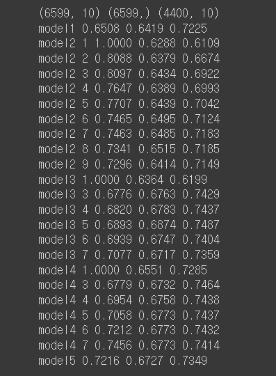
df_OH 사용 모델 만들기 (One Hot Encoding)
# X, Y 분리하기
X2_use, X2_submission, Y2 = get_data(df_OH, Y)
# train, test  7:3 분할, stratify 적용, random_state=0 적용
xtrain2, xtest2, ytrain2, ytest2 = train_test_split(X2_use, Y2,
                                                test_size=0.3,
                                                stratify=Y2,
                                                random_state=0)
# 다양한 모델 만들어 보기
make_models(xtrain2, xtest2, ytrain2, ytest2)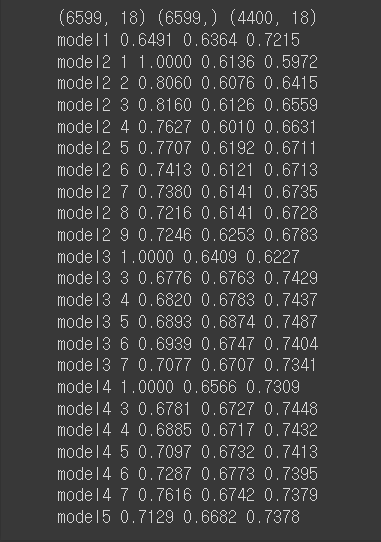
df_MINI 사용 모델 만들기 (One Hot Encoding + 쓸만한 컬럼만 사용)
# X, Y 분리하기
X3_use, X3_submission, Y3 = get_data(df_MINI, Y)
# train, test  7:3 분할, stratify 적용, random_state=0 적용
xtrain3, xtest3, ytrain3, ytest3 = train_test_split(X3_use, Y3,
                                                test_size=0.3,
                                                stratify=Y3,
                                                random_state=0)
# 다양한 모델 만들어 보기
# make_models 함수 호출 부분은
# 실제 시험에서 제출 전에 꼭 주석을 취해 주세요 ^_^  - 실행 시간 초과 금지

make_models(xtrain3, xtest3, ytrain3, ytest3)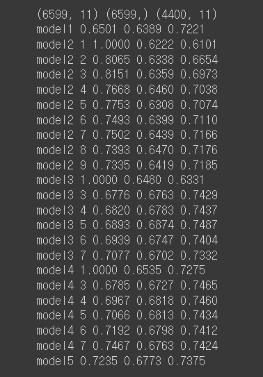
>> 별로 차이가 없지만 성능 좋은것 뽑아서 final model로 다시 생성
model = DecisionTreeClassifier(max_depth=5,random_state=0).fit(xtrain1, ytrain1)
print('final model', get_scores(model, xtrain1, xtest1, ytrain1, ytest1))
4. 제출 데이터 생성
#test 데이터(X_submission, X1_submission)에 대한 확률 구하고 파일로 저장
pred = model.predict_proba(X1_submission)[:, 1]
submission = pd.DataFrame({'ID':X_submission['ID'],
							'Reached.on.Time_Y.N':pred})
submission.to_csv('submission.csv', index=False)

#submission 확인
submission.head(5)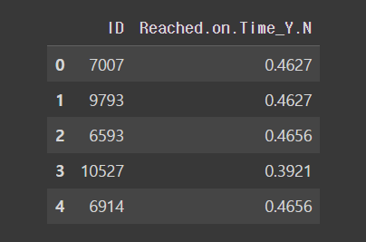
# 아까 생성했던 y_test로 비슷한지 확인 (시험에서는 없음)
ytest = pd.read_csv('y_test.csv')
roc_auc_score(ytest['Reached.on.Time_Y.N'], pred)
#0.7470310932260228
'PYTHON > 빅데이터분석기사' 카테고리의 다른 글
| ML_03 (classification s3-26~30 다항 분류) (0) | 2023.11.15 |
|---|---|
| ML_03 (classification s3-25 이항 분류 모델의 성능평가) (0) | 2023.11.14 |
| ML_03 (classification s3-16~21 작업형 2 예시/고객 성별 예측) (0) | 2023.11.14 |
| ML_03 (classification s3-10~15 분류 모델) (1) | 2023.11.13 |
| ML_02 (Introduction s3-05~09 붓꽃 품종 예측 / sklearn lib) (0) | 2023.11.13 |


